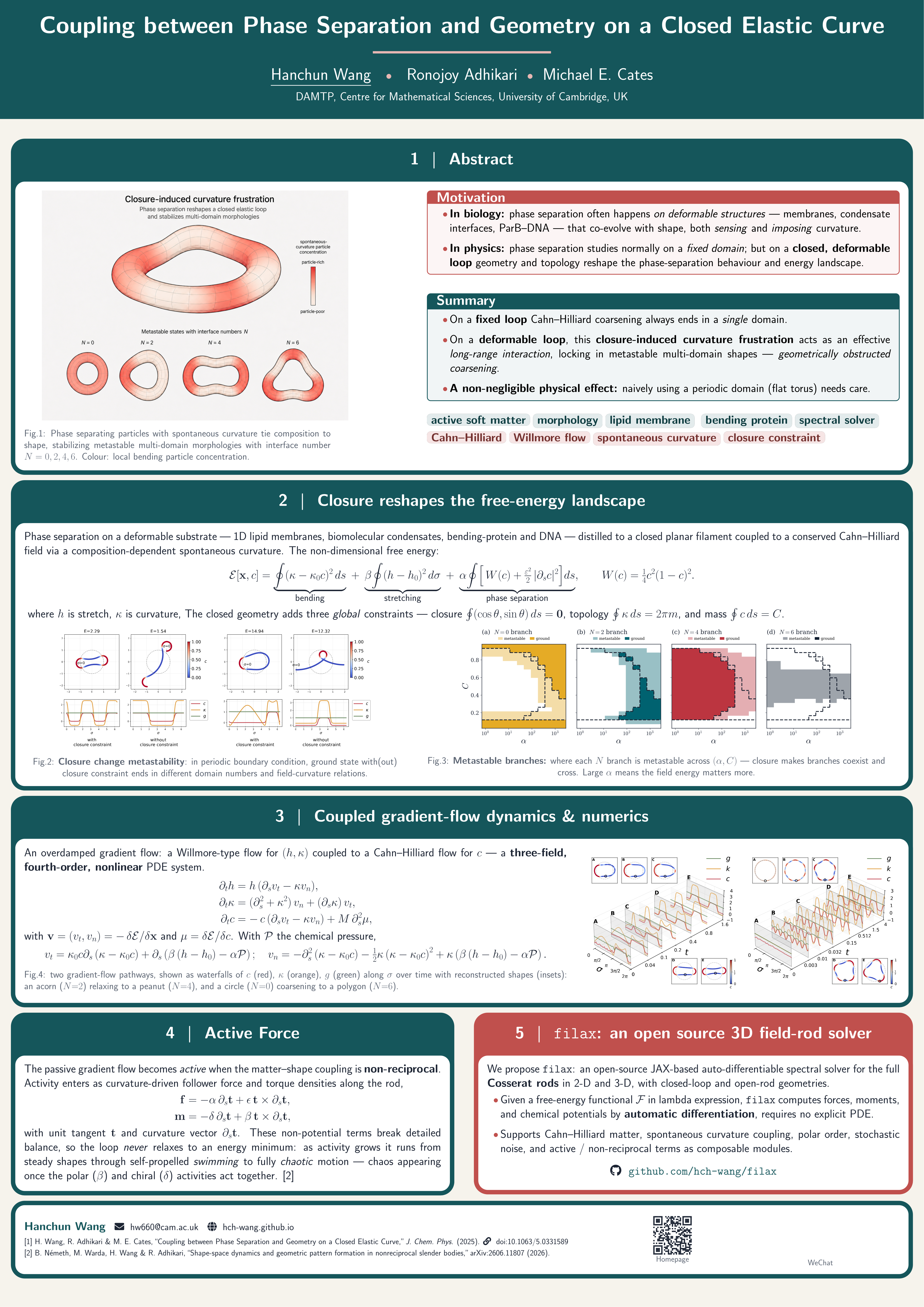
Closure-Induced Curvature Frustration

Phase separation reshapes a closed elastic loop and stabilizes multi-domain morphologies.

Paper

Coupling between Phase Separation and Geometry on a Closed Elastic Curve: Free Energy Minimization and Dynamics

Authors: Hanchun Wang, Ronojoy Adhikari, and Michael E. Cates

Venue: The Journal of Chemical Physics 164, 234902 (2026)

Core Idea

A concentration field $c$ lives on a closed elastic filament. Particle-rich regions prefer curvature $\kappa_0$, while particle-poor regions prefer a flatter shape. Phase separation can satisfy these local preferences, but the loop must still close and accumulate a total turning angle of $2\pi$.

This global constraint makes coarsening nonlocal: merging two domains changes the curvature budget of the entire loop. The competition between interface cost and closure-induced bending frustration stabilizes shapes that would not persist on an open or rigid filament.

Model

The free energy combines bending, near-inextensibility, and Cahn-Hilliard phase separation:

\[\begin{aligned} \mathcal{E} &= E_b+E_s+E_{\mathrm{CH}}, \\ E_b &= \frac{1}{2}\int_{\Gamma}(\kappa-\kappa_0c)^2\,\mathrm{d}s, \\ E_s &= \frac{\beta}{2}\int_{S^1}(h-h_0)^2\,\mathrm{d}\sigma, \\ E_{\mathrm{CH}} &= \alpha\int_{\Gamma}W(c)\,\mathrm{d}s +\frac{\alpha\varepsilon^2}{2}\int_{\Gamma}|\partial_sc|^2\,\mathrm{d}s, \\ W(c) &= \frac{1}{4}c^2(1-c)^2. \end{aligned}\]

Here $\kappa_0c$ is the composition-dependent spontaneous curvature, $h$ measures local stretch, and $\varepsilon$ sets the interface width. Shape relaxation follows a Willmore-type flow, coupled to Cahn-Hilliard transport of $c$ as a three-field, fourth-order nonlinear system.

For tangent angle $\theta(s)=\theta_0+\int_0^s\kappa(u)\,\mathrm{d}u$, a simple closed loop must obey

\[\begin{gathered} \int_{\Gamma} \begin{pmatrix}\cos\theta\\ \sin\theta\end{pmatrix}\mathrm{d}s=\mathbf{0}, \qquad \int_{\Gamma}\kappa\,\mathrm{d}s=2\pi m, \\ \int_{\Gamma}c\,\mathrm{d}s=C. \end{gathered}\]

The closure, turning-number $m$, and conserved-mass $C$ constraints reshape the full free-energy landscape.

Morphologies

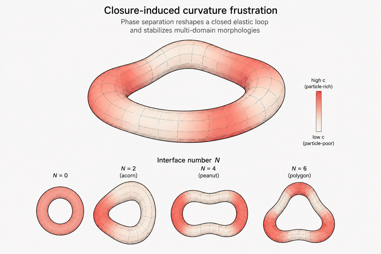
$N=0$ – uniform: no interfaces, but the loop may pay a global curvature-mismatch cost.
$N=2$ – acorn: one interface pair; closure generally forces extra non-circular bending.
$N=4$ – peanut: the smallest generic partition that can satisfy closure with alternating curvatures.
$N\geq6$ – polygon: additional interfaces create higher-energy states that can remain metastable.

Free-Energy Landscape

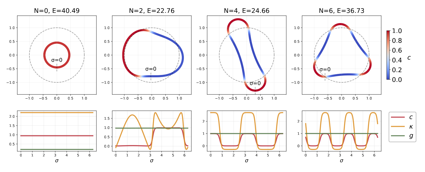
Geometric closure is not equivalent to imposing periodic boundary conditions on the fields. For the same material profiles, enforcing closure changes both the selected domain number and the relation between concentration and curvature.

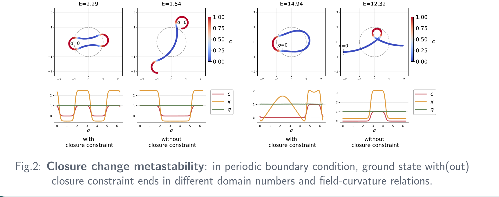
Comparison of equilibria with and without geometric closure — Closure changes metastability. With and without the geometric closure constraint, the minimum-energy state can have different domain numbers and field-curvature relations.

Continuation over field-energy weight $\alpha$ and conserved concentration $C$ reveals overlapping branches with different interface numbers. Their crossings determine which morphology is the ground state and which survive as local minima.

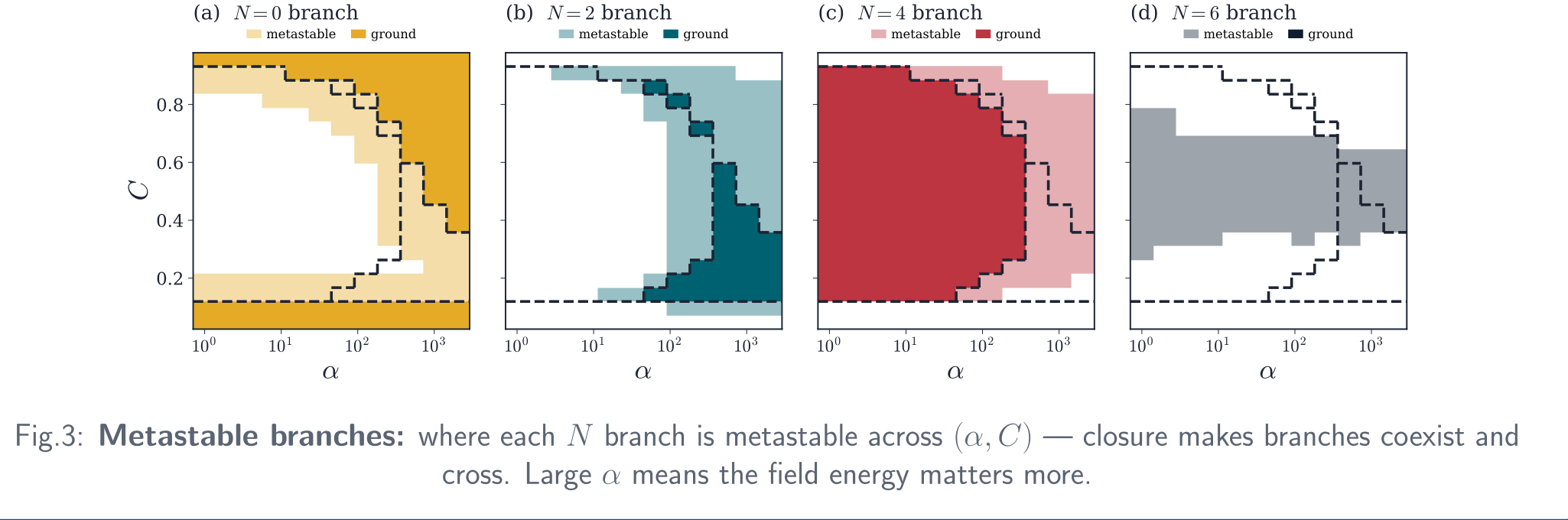
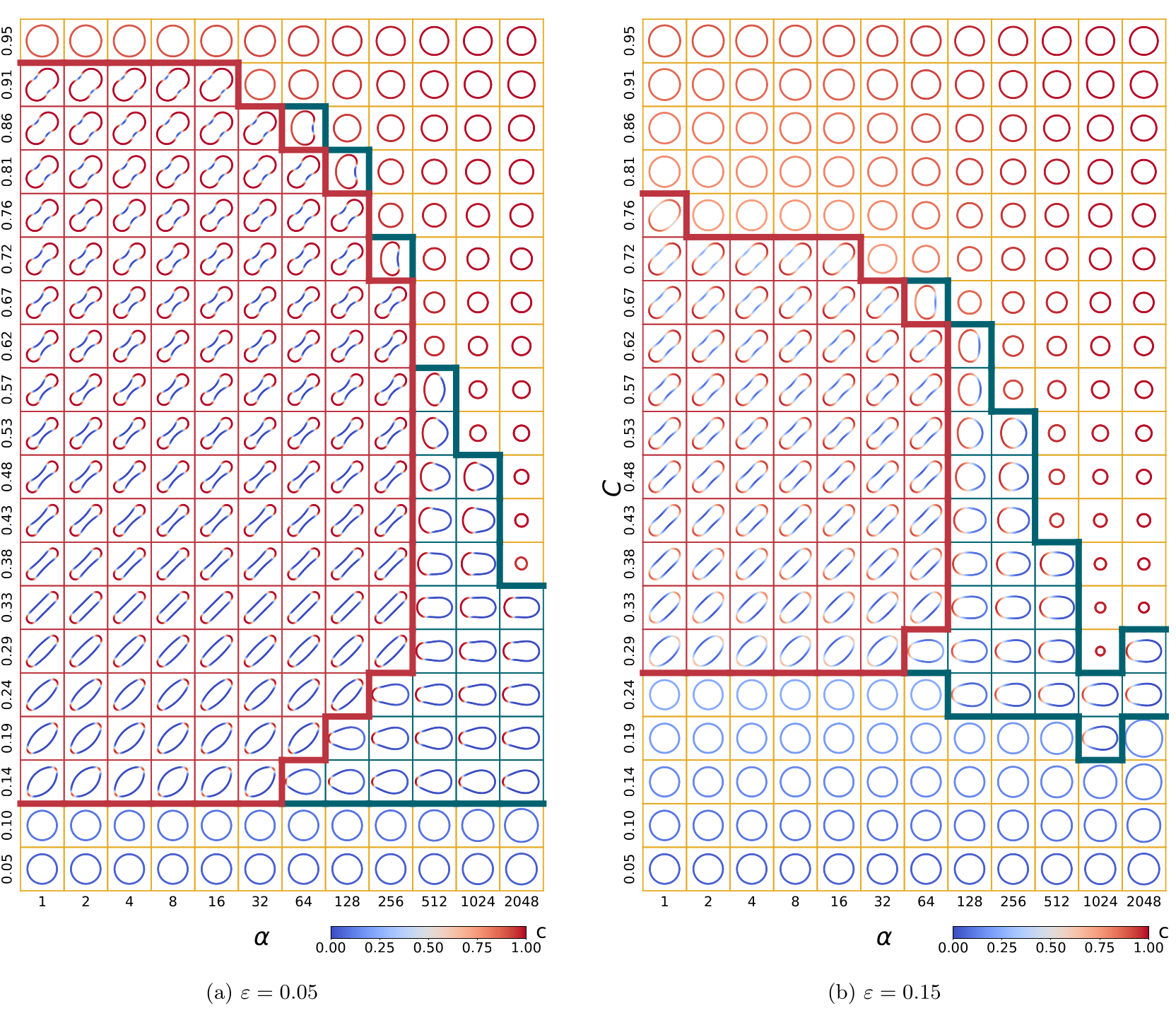
Metastable branches for interface numbers zero, two, four, and six — Metastable regions for the N = 0, 2, 4, and 6 branches across parameter space. Closure makes several branches coexist and cross.

The ground-state phase diagrams show how this branch competition selects the observed morphology. Increasing the interface width $\varepsilon$ raises the cost of interfaces and shifts the optimum toward smaller $N$.

Phase diagrams of minimizing morphologies in alpha and concentration parameter space — Paper Figure 5. Minimizing morphologies in the (alpha, C) plane for epsilon = 0.05 and 0.15. Red and green boundaries delimit the N = 4 peanut and N = 2 acorn phases; the yellow region is the homogeneous N = 0 circle.

Coupled Dynamics

The overdamped evolution couples the filament metric $h$, curvature $\kappa$, and conserved concentration $c$:

\[\begin{aligned} \partial_t h &= h(\partial_s v_t-\kappa v_n), \\ \partial_t\kappa &= (\partial_s^2+\kappa^2)v_n +(\partial_s\kappa)v_t, \\ \partial_t c &= -c(\partial_s v_t-\kappa v_n) +M\partial_s^2\mu. \end{aligned}\]

Here $\mathbf{v}=(v_t,v_n)=-\delta\mathcal{E}/\delta\mathbf{x}$ and $\mu=\delta\mathcal{E}/\delta c$. With chemical pressure $\mathcal{P}$, the tangential and normal velocities are

\[\begin{aligned} v_t &= \kappa_0c\,\partial_s(\kappa-\kappa_0c) +\partial_s\!\left[\beta(h-h_0)-\alpha\mathcal{P}\right], \\ v_n &= -\partial_s^2(\kappa-\kappa_0c) -\frac{\kappa}{2}(\kappa-\kappa_0c)^2 \\ &\quad+\kappa\left[\beta(h-h_0)-\alpha\mathcal{P}\right]. \end{aligned}\]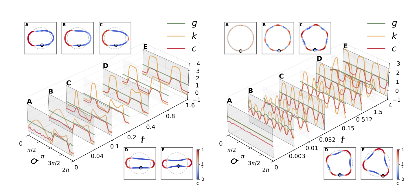

Two coupled gradient-flow pathways on a closed elastic loop — Two gradient-flow pathways. Left: an acorn (N = 2) relaxes to a peanut (N = 4). Right: a circle (N = 0) coarsens to a polygon (N = 6). The waterfalls track concentration, curvature, and metric over time.

Result

On a fixed loop, Cahn-Hilliard coarsening ends in a single domain. On a deformable loop, closure acts as an effective long-range interaction: branches with different $N$ coexist and cross as $\alpha$ and $C$ vary. Coarsening becomes geometrically obstructed and can stop in stable or metastable multi-domain shapes.