Universal Topology Refinement
Model-agnostic topology correction trained with synthetic errors from orthogonal polynomials.
Paper
Universal Topology Refinement for Medical Image Segmentation with Polynomial Feature Synthesis
Authors: Liu Li*, Hanchun Wang*, Matthew Baugh, Qiang Ma, Weitong Zhang, Cheng Ouyang, Daniel Rueckert, and Bernhard Kainz
* Equal contribution.
Venue: Medical Image Computing and Computer Assisted Intervention - MICCAI 2024, Lecture Notes in Computer Science, vol. 15009, pp. 670-680, Springer.
Core Idea
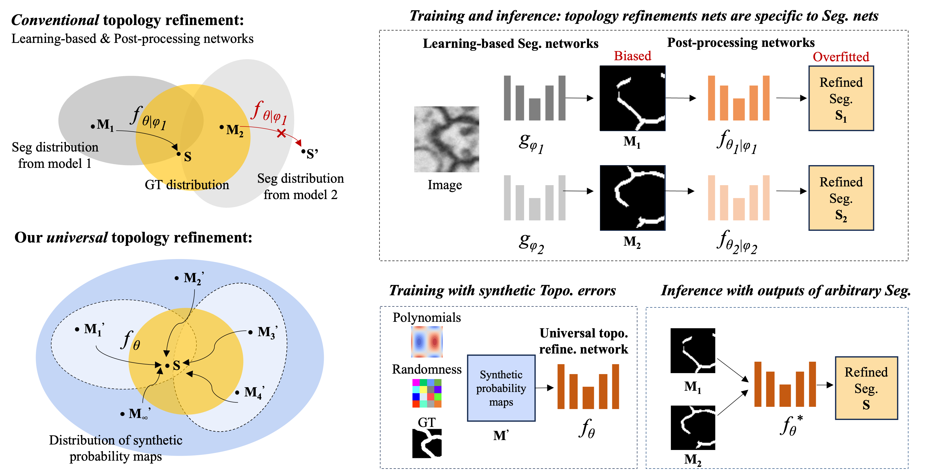
Topology-refinement networks are usually trained on predictions from one upstream segmentation model $g_\phi$. This couples the refiner $f_{\theta\mid\phi}$ to that model’s characteristic error distribution: once $g_\phi$ changes, the refiner can become biased or overfit and must be trained again.
This work breaks that dependency. Instead of collecting errors from a particular segmenter, it synthesizes a broad distribution of plausible probability maps directly from ground-truth segmentations. A single universal refiner $f_\theta$ is then trained on these synthetic errors and can be attached to different segmentation backbones at inference time.
Model
Let $g_\phi$ be any pretrained segmentation network and let $\mathbf{M}=g_\phi(\mathbf{X})$ be its probability map. The proposed post-processing model learns the mapping
\[f_\theta:\mathbf{M}\longmapsto\mathbf{S},\]where $\mathbf{S}$ is a topology-correct segmentation. During training, however, $f_\theta$ never needs predictions from $g_\phi$. Its inputs are synthetic probability maps $\mathbf{M}^{\prime}$ generated from ground-truth labels, so the learned correction is not conditioned on a particular upstream model.
The synthesis starts from a complete orthogonal basis $\Phi={\phi_n}_{n=0}^{\infty}$. A continuous function can be approximated by a linear combination of these basis functions,
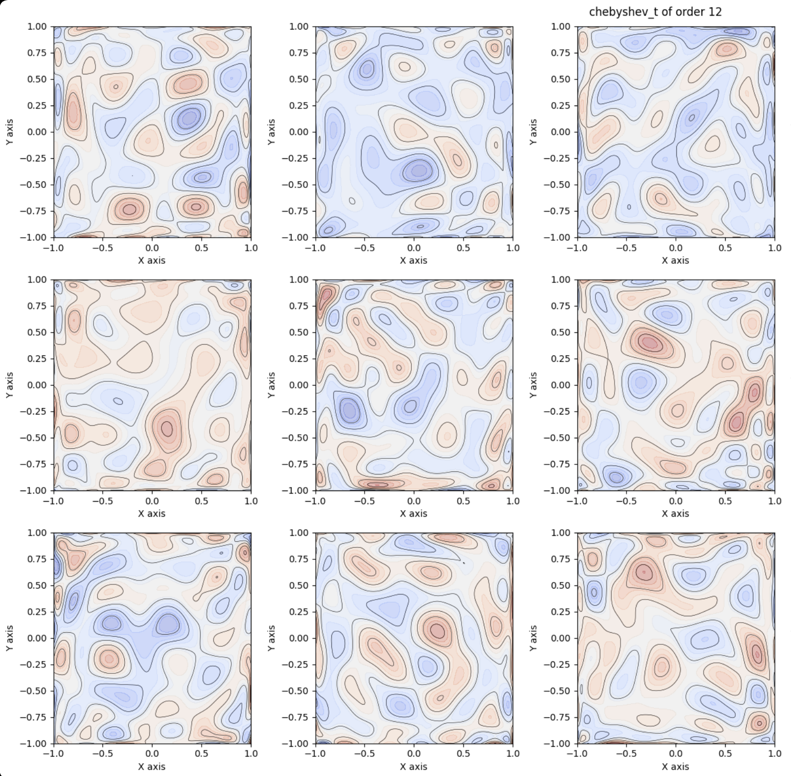
\[p(x)=\sum_{n=0}^{N}a_n\phi_n(x).\]The paper evaluates Legendre, Hermite-Gaussian, and Chebyshev bases. The samples used for this demo are drawn from first-kind Chebyshev polynomials,
\[T_n(x)=\cos\!\left(n\arccos x\right),\qquad x\in[-1,1].\]For a 3D volume, tensor products lift the one-dimensional basis into spatial basis functions:
\[\Phi_{3D}=\Phi\otimes\Phi\otimes\Phi, \qquad e_{ijk}(x,y,z)=\phi_i(x)\phi_j(y)\phi_k(z).\]Synthetic Topology Errors
Random Gaussian coefficients combine the 3D basis functions into a continuous topology-perturbation field, which is the paper’s central synthesis equation:
\[h(x,y,z)=\sum_{i,j,k=1}^{N}a_{ijk}e_{ijk}(x,y,z), \qquad a_{ijk}\sim\mathcal{N}(0,1).\]The order $N$ controls the spatial frequency of the field. Lower orders produce smoother probability variations; higher orders introduce more critical points and can create more complex changes in connected components and loops. The continuous field is sampled at the target voxel resolution:
\[H_{m,n,l}=h(x_m,y_n,z_l) =h\!\left(\frac{m}{N_x},\frac{n}{N_y},\frac{l}{N_z}\right).\]After normalization, the mask $\mathbf{H}$ perturbs a ground-truth segmentation $\mathbf{S}$ by element-wise multiplication:
\[\mathbf{M}^{\prime}=\mathbf{H}\odot\mathbf{S}.\]This operation changes continuous foreground probabilities rather than geometrically deforming a binary mask. When $\mathbf{M}^{\prime}$ is thresholded, its altered critical points appear as realistic disconnections, missing branches, or extra components that the refiner must learn to repair.

Chebyshev Field Demo
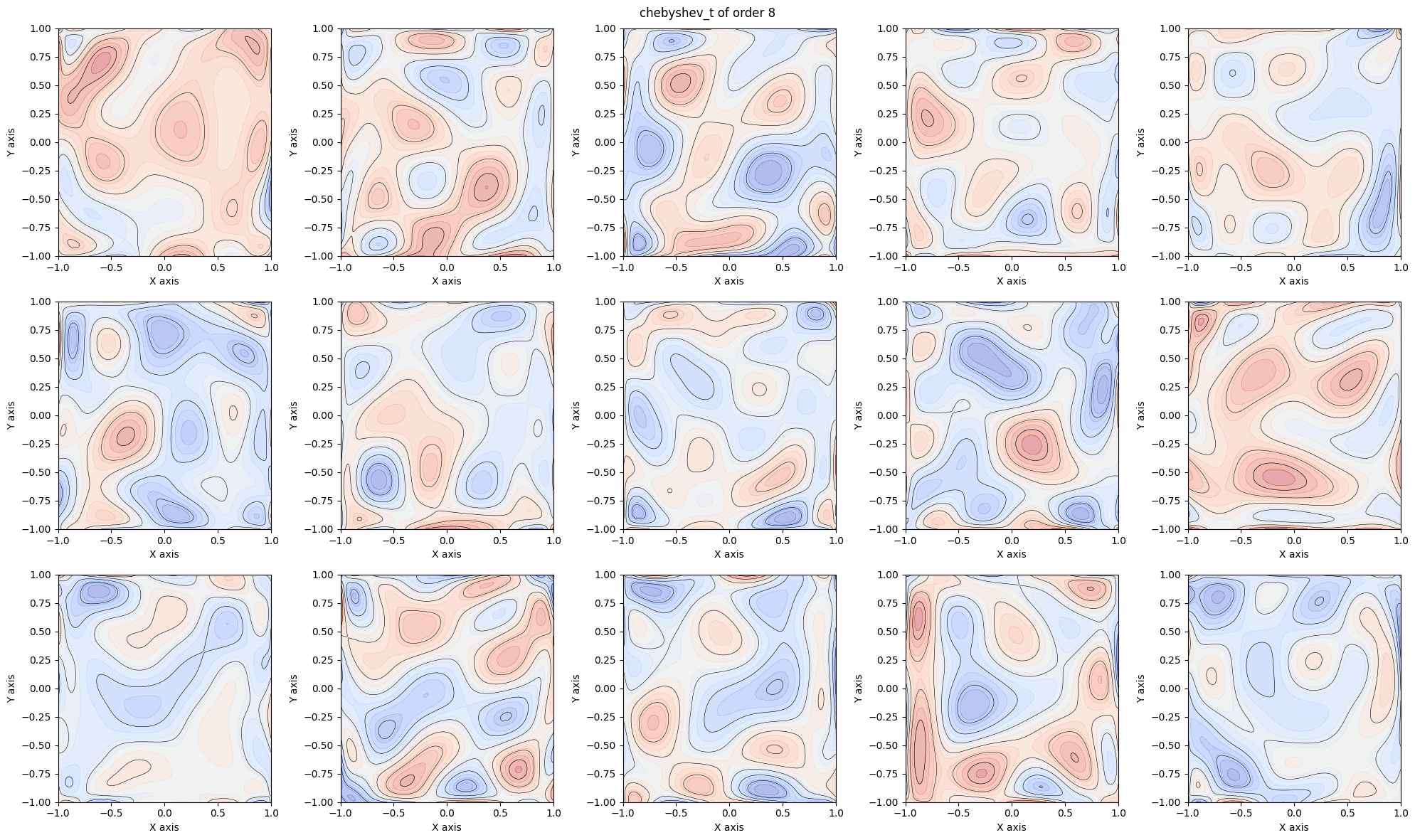
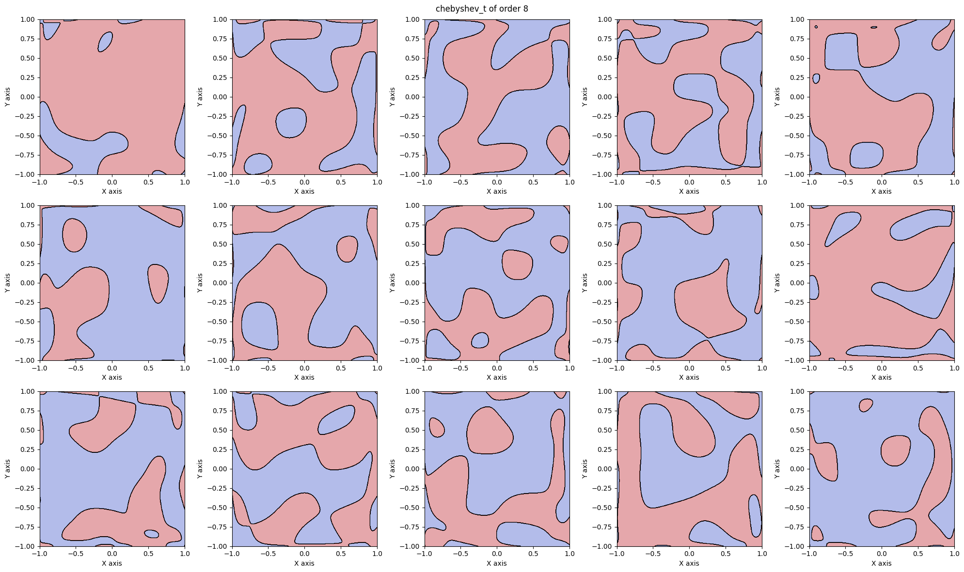
The notebook below samples continuous Chebyshev fields and their binary counterparts using the same polynomial order and random seed.
ps.plot_field_grid(ps.ChebyshevT(), 8, seed=1)
ps.plot_field_grid(ps.ChebyshevT(), 8, seed=1, binary=True)
Open the full Chebyshev notebook
Training and Inference
Training pairs the synthetic map $\mathbf{M}^{\prime}$ with its clean ground truth $\mathbf{S}$:
\[f_\theta(\mathbf{M}^{\prime})\approx\mathbf{S}.\]Additional multiplicative Gaussian noise simulates over-segmentation, while the polynomial masks mainly model smooth topological disruptions. At inference time, $f_\theta$ is frozen and receives the probability map from any compatible segmentation network:
\[\widehat{\mathbf{S}}=f_\theta\!\left(g_\phi(\mathbf{X})\right).\]The result is a plug-and-play topology corrector whose training distribution is defined by controllable synthetic fields rather than the idiosyncrasies of one segmentation backbone.